Introduction:
The dataset used in this project, “Slave Sales: 1775-1865”, includes information that is numeric, textual, and geographic, which was used to create two data visualizations utilizing TableauPublic. There are thousands of people in this list from mostly Southern States, including Georgia, Louisiana, Maryland, Mississippi, North Carolina, South Carolina, Tennessee, and Virginia. To differentiate the states, there are thirty-six different counties, which seem to have some importance as to where slaves with certain skills are sold. In terms of numeric values, these fit into the year of sale, appraised value, and age columns. The year of sale column actually starts in 1742, with one entry, but becomes consistent after 1771, even though the title of the dataset begins with 1775, and ends in 1865. The minimum values for the other two columns both start at zero, but the maximums vary greatly. The maximum age of a given individual can go up to 99, but this is most likely a reporting error due to the fact that it is unlikely that someone could live to that age during this time period. The price for a person also depends on skills and other factors, and the highest price for a slave sometimes exceeded thousands of dollars (again, there was one outlier, a slave listed at $525,000, which would be more than $7 million when adjusted for inflation). The range of descriptive data also varies greatly. Gender is probably the easiest to describe as it follows a binary system, with a slave being either male, or female. The column titled “Skills”, however, is either left blank, or provides a short description about the person. These skills can either show if someone is a field-hand, which is the most common profession for slaves (excluding the “null” descriptor), or if they have specialized training as a carpenter, mechanic, or hairdresser. As stated above, skills determined how much a slave was typically worth, with unskilled laborers usually fetching a lower priced than their skilled counterparts. Issues do reveal themselves, as the large number of slaves with the nothing listed in their skill column create problems. This happens because the highest price of a slave with a skill listed is as blacksmith worth $3500, which is problematic, as appraised values continue to rise from here without any description of what the slave’s skills are. The last column, “Defects”, lists any physical or mental problems a slave might have. These include slaves suffering from things like a hernia, crippling injuries (an example: missing fingers, most likely due to a cotton gin), on the physical side of descriptors, or being deemed insane, or mentally unsound. There are also issues such as alcoholism (labeled as suffering from consumption), and other ailments that are strange (one slave apparently being a “dirt eater”). One interesting feature in this dataset is how there are labels for “boy” or “girl” when no other relevant information is listed for the slave. In cases like these, the age listed shows “0”, for both years and months. This may indicate that the person for sale has not been born yet, which adds another horrifying layer to this dataset, as even the unborn are for sale if this is true. Another possibility is that the data is incomplete, and that these are only typos or information that was excluded in the sales listing.
First Visualization Description/Problems:
The first piece of data visualization is a line graph comparing the median “appraised value” of men and women in skills where both sexes intersect. Out of the sixty skills that are listed in the dataset, women are listed in twenty, and out of these twenty, at least half are learned trades. This was surprising, as that meant women appeared in a third of the listed skills. In addition to this revelation, women also received training in about ten learned skills, which is amazing considering that there were already only a few skilled professions that slaves learned according to the dataset.
In addition to this revelation, women sometimes exceeded their male counterparts in “appraised value”. This occurred with female liquor distillers, drivers, gardeners, hair dressers, laundresses, and tailors, or over a quarter of the listed skills. The average appraised value of women was also $535.25 versus the averaged amount of their male counterparts, which comes out to $588.65 when calculated. The original expectation of this project was that men would far exceed women in median “appraised value”, but this did not happen. Instead, men only exceeded women by a little more than $50 when the median values were averaged together. Another interesting point in this visualization are the peaks and valleys between certain skills. In terms of female slaves, there are several places where the median “appraised value” of women exceeds men by over $350. These peaks occur with drivers, hairdressers, and tailors for women, and for men, they peak with only mechanics and seamstresses. Another interesting part of this is that when the highest peaks for men and women are compared, hairdressers and mechanics, the difference is surprising. While male mechanics are worth more than female hairdressers, when you compare the opposite sex in these two skills (male mechanics:$1200 vs female mechanics:$600, and male hairdressers: $275 vs female hairdressers:$1000), the hairdressers have a larger divide between them. While this may be inconsequential, the fact that hairdressers were valued almost as much as mechanics is incredibly amazing. In spite of this, women were consistently appraised at a lower price than men, which is seen in the skills that are not used in this visualization. There is also the fact that while men sometimes worked in what could be considered a female profession, this kind of cross-over did not occur with women. As stated above, there are sixty skills listed in the dataset, and while women do occupy a third of them, there are only a few outside of these that women are listed under, which are dairy, midwife, nurse maid, and spinner. Meanwhile, male slaves occupied more skills that would be likely to fetch a higher price at a slave market, such as black-smithing, and other trades. I also imagine that, in addition to the already horrible amount of racism present in the South at this time, the hardships that a female slave would have to endure would have been worse, and that this racism and sexism probably prevented women from receiving training in certain skills.
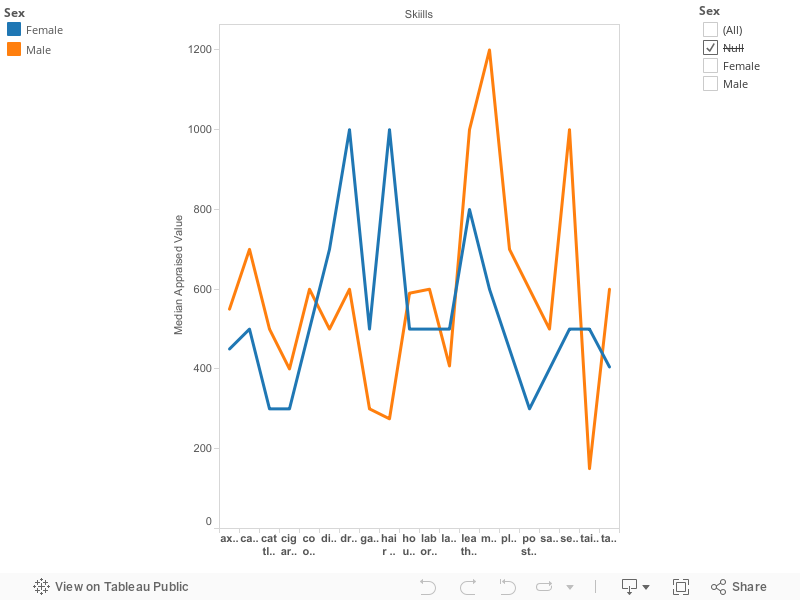
For the line graph visualization, specifically, a number of different graphs were considered before this one was settled upon. The first version of this visualization involved the use of a bar graph, and more professions, but this proved difficult to understand. The main issue with the bar graph came from the fact that it stacked the values on top of each other, which created an awkward presentation of data. This format made it appear unclear as to whether or not there was any deviation in value between the sexes. It also created problems for measuring the median “appraised value” in each skill, as the stacking made it unclear as to which sex was being measured. After this, the line graph was chosen because the sexes were represented by two differently colored lines, solving the issue of indistinguishable data points, while also creating a clearer visualization for the average viewer. A pie chart was also considered, but that came with its own set of issues, so it was scrapped early on in the development of the visualization. This is also the second version of the line graph visualization, but there were still issues present within the graph. In the case of female skinners and shipbuilders, there were problems with the data, as the values were extremely low, which happened with the female skinner, as she was listed as being appraised as $0, with a similar problem happening with the shipbuilder who was for sale for $5. These two professions were statistical outliers, and were excluded from the data because they threw off the overall data. Other groups were also excluded, but for different reasons. The skills: “null”, “no talent”, and does a bit of all, good character”, all appear multiple times , but provide little to nothing in the way of description for the person it is attached to. This caused frustration, especially with the “nulls”, as slaves with named skills never exceeded more than a certain amount of money, while the “appraised value” of “nulls” continued to rise. Conversely, some of the intersecting skills contain many listings for $0, like the female skinner. This isn’t seen as clearly, as there are more people trained in these skills that counterbalance the “zeroes” (the female skinner was the only one). Some other problems are related to the definitions of certain skills in the modern era. While the skill, “driver”, might have a clear meaning in the 18th and 19th centuries, for people in the modern age, there are some difficulties. In this case, driver can refer to a skill similar to a cartman (a carriage driver), an overseer (slave driver), or a cattle minder (cattle driver). All three of these present possible definitions, but the true meaning of the driver’s skill remains unclear. (note to Dr. Kane: I did look up when the word driver ,as related to cattle driver, was first mentioned according to the Oxford English Dictionary, and it turns out that it happened in 1483, so I was incorrect).
Second Visualization Description/Issues:
The second visualization provides details about slaves with listed skill-sets, and which states/counties they were more likely to be located in when their abilities were taken into account. The maps create a striking narrative, with Louisiana, the state deepest South, containing more unskilled slaves than almost every other state. This can be seen in the maps pertaining to common laborers/field-workers, plowmen, and woodcutters/sawyers. In contrast to this, skills that required some sort of formal training, such as coopers, carpenters, and tailors/seamstresses, can be found outside of Louisiana in larger numbers. However, there are a few cases where slaves with training in certain skills did appear in higher quantities in Louisiana than other states. This occurs with slaves who received training as mechanics, cooks/pastry chefs, and brick masons. There is another skill that could fit into this category, blacksmiths, but there are a couple of reasons this one is excluded. The first reason is that Louisiana contains a disproportionately high amount of slaves when compared with the rest of the South. A feasible explanation for this relates to the amount of trade Louisiana, especially in New Orleans, participated in during the Antebellum period. In the years preceding the Civil War, New Orleans generated high amounts of revenue from its involvement in trade, exporting millions of dollars worth of products (Clark, 131). The invention of the cotton gin in 1793 also increased the demand for slaves to pick cotton in the Northern parts of the state, while sugar cane continued to dominate in the rest of Louisiana. This explains the extremely above average numbers of laborers/field workers, and could explain the mildly above average number of brick masons and mechanics, as they would be needed to support the growing number of slave plantations in the state. Explaining the number of coopers and carpenters in Charleston County, South Carolina may pose a more difficult challenge. During the late 18th and early 19th centuries, Charleston, the city, existed as a major port and trade center, but in the waning years of the Antebellum period, evidence of decline began to appear (Zierden and Calhoun, 29). This could explain the higher than average number of coopers, as barrels would be used to ship certain products, like rum or molasses. Similarly, the high number of carpenters probably grew out of necessity as well, as Charleston suffered from frequent fires and hurricanes, meaning that it would be desirable to train slaves in this trade when people inevitably had to rebuild their homes in the wake of disaster (Zierden and Calhoun, 35-36). While these may not be the exact reasons that there were more carpenters and coopers in the area, it seems reasonable to assume that under these circumstances, it could be possible.
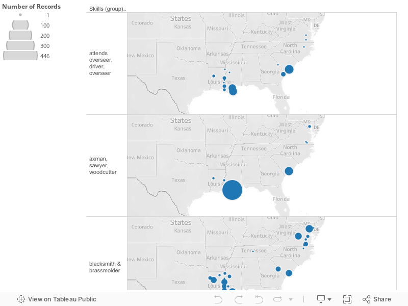
Similar to the line graph visualization, a number of different versions of this map were made before the final one was settled upon. In the early stages of the project, the original intent was to show which states had large amounts of slaves with learned trades. There were problems with this approach, as there were either issues with skills having only a handful of people trained in them, which made presentation difficult, and made the act of drawing conclusions difficult. The other problem with the data came from the fact that a large amount of slave sales occurred in Louisiana, while there may not have been as much in other states. In order to rectify these problems, skilled and unskilled laborers were included as long as the number of entries exceeded a certain threshold, and certain skills that only appeared in Louisiana were excluded entirely. When this was done, a narrative appeared, showing that Louisiana had a large amount of unskilled laborers, while other states, such as Maryland and South Carolina had more slaves who received training in certain trades. This made the data easier to interpret, along with creating more interesting visualizations, showing the stark contrast between Louisiana and the rest of the South, as stated in the previous section.
Other problems had more to do with how the data could be presented as opposed to the data itself. Before the differently sized dots was settled upon, there were a number of different attempts made to present the data. The first attempt used gradient colors to show the difference between states/counties with large slave populations, but this came with a number of issues. When this format was used, there was little difference between the counties that had large slave populations and those that only had a few. When I figured out how to fix the amount of variation between shades, it created problems with interpretation. If a typical viewer looked at one of the visualizations, he or she might not be able to figure out what the different colors represented. The dots were chosen to fix this problem, and they do make the data easier to interpret, with larger dots showing larger populations of slaves, and smaller dots doing the opposite.
There were also some smaller problems that were easily rectified. In one instance, the names of two counties (Ouachita Parish, Louisiana and Rutherford County, Tennessee) were entered incorrectly, causing Tableau Public to read the sales from the counties incorrectly. The fix for this involved finding the correct names for the counties, and reentering the correct spellings. Another small problem appeared when I mistakenly changed the geographic section of the data from county/region to country/region, which caused the data points to appear in the middle of the Atlantic Ocean, or in Eastern Europe (Georgia, the country, versus Georgia, the state). The final small problem related to skills with similar spellings or definitions. In this case, defined skills, like “laborer of fieldwork” did not combine automatically with “laborer or field work”, even though the two different skills were actually the same. The solution to this problem was easy, and similar skills were put into categories with each other.
Broader Historical Context:
In terms with how the data intersects with broader historical patterns, there are a number of conclusions that can be drawn. One of these conclusions is that, as time went on, slave sales began to rise in the Deep South while they declined closer to the Mason-Dixon Line. This can be seen especially in Maryland, which controlled much of the slave trade in the late 18th and early 19th century. This may not be clear from the visualizations I have provided since “nulls” are excluded, but when they are accounted for, it’s obvious that Maryland participated heavily in the slave trade. This changed after the late 1820s and into the 1830s,and the slave trade moved deeper into the South. Maryland, in contrast with the rest of the South, would be the only state in this list to not secede from the Union during the Civil War, and by 1860, almost half of the state’s African-American population consisted of free blacks (Kolchin, 81-82). It should also be noted that while Maryland made slavery illegal in 1864, it appears that, at least according to the information provided in the dataset (and from my own examination), that Maryland stopped trading slaves after 1853 (1853 appears to have been the last year people participated in the slave trade, so there were a large amount of listings before the state dropped from the dataset entirely). After Maryland’s participation began to decline, Louisiana, and to a lesser extent, South Carolina and Georgia, began to dominate the trafficking of enslaved persons, while North Carolina and Virginia were consistent, but not nearly as prolific. This trend can be clearly seen up until the end of the Civil War in 1865, where the dataset ends, with a few exceptions.
Another conclusion that can be drawn, at least from the data visualizations, is that the South never seemed to diversify from its agrarian roots, while the North would dominate industry during this period. This can be seen in the large amount of slaves sold as field workers compared to the number of slaves trained in skilled trades, especially in Louisiana. While it was shown above that there were average numbers of mechanics and brick masons, these numbers could not compete with the extraordinarily high amounts of house servants, laborers, and woodcutters. In states like Louisiana, which relied on the harvesting of sugar cane for much of its agricultural revenue, it would make sense to have higher concentrations of field workers in order to harvest crops. Mechanics would also only be needed in places with certain types of technology, so having a certain amount in areas like New Orleans would make sense, as the city was a central hub for trade on the Mississippi River. This means that machines like steamboats would travel back and forth on the River, and make port frequently in New Orleans, so having mechanics on hand to repair these ships could be a possibility for why there were slaves trained as mechanics in the city. The relatively low density of mechanics can be explained on a supply/demand basis when compared with field workers, as it may not be as necessary to have more mechanics during this time, at least in the view of slave owners in Louisiana. In order to draw more contrast, and elaborate on this idea, I would like to point out that the number of blacksmiths in Virginia and Maryland. This is one the only times that these two states have more slaves with a defined skill-set than Louisiana and South Carolina (the other case involves carpenters, which will be touched upon in the next section). This shows the divide between the Upper Southern States and the Deep South because even though slavery was still used in states like Maryland, there was at least the hint of a movement away from an agrarian way of life that other Southern states desperately wanted to continue.
In terms of how female slaves were treated, it’s difficult to make assumptions based on the data alone, but there are some striking differences that can be seen. As stated in the description for the first visualization, women appear in about twenty listed skills, excluding “null”, “no talent”, and “does a bit of all, good character”. While most of these intersect with the opposite sex, the number of women occupying these positions was rather low, and in examining the data, the viewer can see that female slaves were used mostly for fieldwork or as house servants. This doesn’t devalue the inherent value of skills like hairdressers, it’s just that there were only two female hairdressers in the entire dataset, so the percentage was low when compared with everything else. This segregation can have a number of reasons, but it was most likely caused by a combination of sexism and racism that was prevalent during this time. While white women were probably expected to not participate in activities that were considered masculine, the same most likely followed for female African-American slaves, albeit in a less genteel fashion, as the gender difference didn’t matter in regards to back-breaking labor. When combined with racism, it was probably assumed the female slaves lacked the mental proficiency/capacity to learn skills like black-smithing, masonry, or carpentry. Again, this isn’t saying that just because women received training in other skills that they aren’t as valuable, but there is a clear difference in “appraised value” between men and women. However, this didn’t stop a few women from learning what could be considered masculine trades, as there was at least on female slave who received enough training to be listed as a mechanic in the New Orleans area in the middle of the 1840s. While this is only one person, and I would rather not call it progress because she was still enslaved, it is possible that towards the middle of the nineteenth century, some African American women began learning more masculine trades.
Further Research Questions:
There are also many other questions that this data brings up that could not be included in this project. I’ll attempt to explain the reasoning behind some of my questions to the best of my ability. The list is as follows:
Did slave revolts have any impact on the number of listings for certain years, or could the declines be explained as the result of other occurrences?
If carpenters were predominantly located in a city like Charleston as a result of necessity after fires or natural disasters (hurricanes), would it be possible for other large concentrations of carpenters to be located near other cities for the same reason?
Were skilled laborers worth more than unskilled laborers?
Why does it appear that some skills were valued more than others? Why would a hairdresser be worth almost as much as a mechanic? I’m not saying this to belittle either one, it just surprised me is all.
How do the “nulls” impact this dataset? Would it be possible to fill in some of the gaps that exist here?
Would it be possible to figure out which occupation “driver” refers to with more research? I only ask this because I was unable to settle the matter myself, as the word has more than one possible meaning in the context of the dataset.
Did the age of slaves impact their “appraised value”? Another question I didn’t have time to answer, that I think Alicia may have touched upon in her project. This would have been part of the median sale price visual, but again, time constraints.
How did the invention of the cotton gin affect the number of defects found in slaves? I noticed that a few listings had notices of the people they described lacking hands and in one case an arm, and I wonder if these became more prevalent as time went on.
The first question I will attempt to elaborate upon is if slave revolts during this time had any affect on the slave trade. During the Antebellum Period, there were many notable slave rebellions occurring in the South, most of which were unsuccessful. In the timeframe of the data, there were several notable revolts in the United States, which included the German Coast Uprising in 1811, Nat Turner’s Rebellion in 1831, and John Brown’s Raid in 1859. While there were a few other revolts, these three were much larger in scope and size, with the exception of John Brown’s Raid, which, while small compared to the other two, had larger implications as it heightened tensions in the South a year before the Civil War began.
The German Coast Uprising, which occurred in January of 1811, involved between 100-200 slaves, with some estimates as high as 500, depending on the source (Kolchin,156), who worked on sugar plantations, and may have been inspired by the Haitian Slave Revolution that ended a few years before the Uprising. While it may be a stretch, there appears to be a steep decline in the amount of slave sales conducted in Louisiana during 1811, at least according to the available dataset. This decline can be seen after 1810, which has a normal amount of sales, and in 1812, when the number of listings rebounds. This occurrence also appears to happen in Virginia after Nat Turner’s Rebellion in 1831, but it’s a little more difficult to draw this conclusion because Virginia’s participation in the slave trade appears relatively low, at least during the late 1820s and early 1830s. It seems entirely possible that slave owners might be wary of selling or purchasing new slaves in the aftermath of a major slave revolt, for fear that it could happen to them. Additionally, to make sure that these declines weren’t caused by economic upheavals, I double-checked when these occurred, and the closest recessions I found were the Panics of 1819 and 1837, which ruled out this possibility. Whether or not the two are related, it would be interesting to see if this question could be taken somewhere by someone with expertise in this subject.
Going in a different direction, I think it would be interesting to see if other states/counties had more slaves trained in carpentry suffered from frequent fires. Since I concentrated exclusively on Charleston County, South Carolina, that meant I didn’t give time to other places with slightly lower numbers of carpenters. These places included Anne Arundel County, Maryland, located between Baltimore and Washington, D.C, the Orleans and Plaquemines Parishes in Louisiana, and Chatham County in Georgia, which contains Savannah. Each of these counties either housed or was in close proximity to a major city, and during this period, fires destroying parts of cities appears to be commonplace. Within the time of the dataset there were a two fires that received documented attention outside of one that happened in Charleston in the late 1830s. The first was the burning of Washington, D.C in 1814 during the War of 1812, and a fire that happened in Augusta, Georgia in 1829. While there may be less reason to assume that the capital required carpenters for the more important buildings (the White House and Capitol building survived; Herrick, 91), which were constructed from stone, it is likely that there were other structures that needed to be replaced. Augusta, in contrast, lost as many as 850 homes when a fire ripped through the city in the spring of 1829, most likely requiring people with expertise in carpentry to aid in rebuilding. Going off of this question, a more experienced researcher might be able to find more connections with the geographic distribution of other skilled laborers, and why they ended up in certain areas.
Another question I wanted to explore, but ran out of time to do relates to the median appraised value of skilled and unskilled slaves. While I was able to work out the difference between men and women, I was unable to figure out how to present skilled versus unskilled slaves. When I first started this project, I assumed that skilled laborers would have a higher median “appraised value” than their unskilled counterparts. This didn’t appear to be the case, and as I delved further into the data, it seemed that the overwhelming amount of slaves who were sold as common workers skewed the data in the opposite direction. This was surprising, but when I compared field workers to carpenters, I found that the fieldworkers were consistently valued between $300-$800 while carpenters varied more wildly. Given more time, I might have been able to come to a more defined conclusion, but this wasn’t the outcome, which is unfortunate because there seemed to be an interesting underlying story between these two groups.
As stated in an earlier part of this post, the high number of “nulls” has been a consistent frustration for me in trying to examine this dataset. As a whole, “nulls” account for the largest category under the “skills” column in “Slave Sales:1775-1865”. These blanks make me feel like the data is incomplete, and its impossible to ignore because of the fact that this group makes up the majority of slave sales in all of the states included in the dataset. That makes this gap more of a chasm than anything, which is why I wondered if the possibility existed of making the data more complete. While there are ways of interpreting the “nulls” based on other values, mostly their age and “appraised value”, which could be mutually exclusive in some aspects as it appears that younger slaves received higher appraisals than older slaves in some cases. In spite of this, the gaps that exist mean this data is still lacking when compared with the listings that contain more relevant information.
Conclusion:
In conclusion, this project has given me a whole new appreciation for how horrible slavery was in the South during the Antebellum period. In seeing the thousands of people listed in the “Slave Sales:1775-1865” CSV as you might see items in a “Want Ad” in the newspaper, the enormity of a situation I understood, but never fully comprehended became much more prescient in my mind.Reducing a fellow member of the human race to a number based on age, sex, skill, and defect feels wrong. This isn’t to say that I didn’t learn anything from examining the dataset, on the contrary, it either confirmed some of my own ideas, and caused me to think about solutions to problems that were brought up in class. It’s just a uniquely horrible experience to write about slaves as things, rather than people.
Bibliography:
Calhoun, Jeanne and Zierden, Martha, “Urban Adaptation in Charleston, South Carolina, 1730-1820”, Historical Archaeology, Vol. 20, No. 1 (1986), 29-43.
Clark, John G., “The Antebellum Grain Trade of New Orleans: Changing Patterns in the Relation of New Orleans with the Old Northwest”,Agricultural History, Vol. 38, No.3 (July, 1964), 131-142.
Herrick, Carole, August 24, 1814: Washington in Flames, (Falls Church, VA: Higher Education Publications, Inc, 2005).
Kolchin, Peter, American Slavery: 1619–1877 (New York: Hill and Wang, 1993)
Georgia History Timeline / Chronology 1829, Our Georgia History, accessed May 9, 2016. http://www.ourgeorgiahistory.com/year/1829